Machine Learning : Decision Tree
Intro#
 aG(x)=c=1∑C[b(x)=c]Gc(x)
Basic Decision Tree Algorithm#
當還未滿足終止條件時,執行 :
- 學一個分割準則 b(x)
- 當前節點分割 : D to C parts Dc={(xn,yn):b(xn)=c}
- 分割出來的子集再做遞迴呼叫 : Gc←DecisionTree(Dc)
- 返回當前節點的預測函數 : G(x)=∑c=1C[b(x)=c]Gc(x)
C&RT (Classification and Regression Tree) Algorithm#
Branching#
- 選擇最佳分割準則
- 總是創造二元樹
- 基於leaf的最佳常數 : gt(x)=Ey∣optimal constant
Purifying#
- 用一個簡單的閾值做二元分類
- 純化節點 : b(x)=decision stumps h(x)argmin[Dc with h]⋅impurity(Dc with h)
Some Metrics#
- Regression Error : impurity(D)=N1∑n=1N(yn−yˉ)2
- Classification Error : 1−max1≤k≤KN∑n=1NI(yn=k)
- Gini Index : 1−∑k=1K(N∑n=1NI(yn=k))2
Algorithm#
- 學一個分割準則 : b(x)=decision stumps h(x)argmin[Dc with h]⋅impurity(Dc with h)
- 考慮最佳的樹樁 : Dc={(xn,yn):b(xn)=c} ,切出兩個子集
- 遞迴
- 返回組合之後的模型 : G(x)=∑c=12I(b(x)=c)Gc(x)
Regularize#
- Pruning
- 做決策樹時,同時把複雜度加入懲罰項
- 先長出完全樹,再去每一步選擇能最小化 (Error + 複雜度) 的node
Branching on Categorial Features#
- 可以根據出現率 / label相關性排序,再做類似數值特徵的閾值分類
Surrogate Branch#
- 關鍵的特徵剛好缺值
- 在訓練時對每個 b(x) 就先算一次次要分裂,想辦法用其他特徵構造出效果差不多的樹樁
- 遺失資料時可以用替代路徑做分類
Properties#
決策樹優勢#
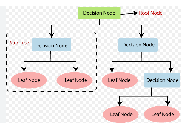
- 易於理解和視覺化
- 能處理數值和類別特徵
- 自動特徵選擇
Adaptive Boosting#
Boostrap (Re-Weighting)#
- 對原始資料做抽樣(有重複,不平均)
- 每個Learner想辦法最小化誤差
如果每次只是隨機Boostrap,Base Learner會太相似,重採樣強迫學習不同的解
Optimal Re-Weighting#
- 假設當前Base Learner的錯誤率是 : ϵt=∑nun(t)∑nun(t)I[yn=gt(xn)]
- 我們希望更新權重之後對錯各半,因此 :
- 錯分的資料乘 (1−ϵt)
- 分好的資料乘 ϵt
- Normalization
- Scaling Factor : ϕt=ϵt1−ϵt
依照Scaling Factor的定義,假如當前Base Learner的效果很好,則會把錯分的資料加權到超大,把注意力轉移到更難分類的樣本
AdaBoost Algorithm#
- 先初始化權重(一開始大家都一樣) : un(1)=1/N
- 進行迭代 :
- 訓練弱分類器 gt ,最小化 ϵt=∑n=1Nun(t)∑n=1Nun(t)I[yn=gt(xn)]
- 計算 ϕt=(1−ϵt)/ϵt,更新權重 u(t)→u(t+1) :
- 分類錯誤的權重乘以 ϕt
- 分類正確的權重除以 ϕt
- 令 αt=lnϕt (越準確的 gt,αt 越大),越大代表在最終決策有更大權重
- 最後輸出分類器 :
G(x)=sign(∑t=1Tαtgt(x))
Decision Stump as Base Learner#
- 做一個簡單的樹樁來二元分類 : h(x)=s⋅sign(xi−θ)
- 目標是找最佳的分裂方向,可以先對特徵值進行排序
- 暴力搜索參數((θ,i,s)),總複雜度是 O(d⋅NlogN)